Posts tagged "research":

A simple thread pool to run parallel PROSail simulations

In the otb-bv we use the OTB versions of the Prospect and Sail models to perform satellite reflectance simulations of vegetation.

The code for the simulation of a single sample uses the ProSail simulator configured with the satellite relative spectral responses, the acquisition parameters (angles) and the biophysical variables (leaf pigments, LAI, etc.):

ProSailType prosail;
prosail.SetRSR(satRSR);
prosail.SetParameters(prosailPars);
prosail.SetBVs(bio_vars);
auto result = prosail();

A simulation is computationally expensive and it would be difficult to parallelize the code. However, if many simulations are going to be run, it is worth using all the available CPU cores in the machine.

I show below how using C++11 standard support for threads allows to easily run many simulations in parallel.

Each simulation uses a set of variables given in an input file. We parse the sample file in order to get the input parameters for each sample and we construct a vector of simulations with the appropriate size to store the results.

otbAppLogINFO("Processing simulations ..." << std::endl);
auto bv_vec = parse_bv_sample_file(m_SampleFile);
auto sampleCount = bv_vec.size();
otbAppLogINFO("" << sampleCount << " samples read."<< std::endl);
std::vector<SimulationType> simus{sampleCount};

The simulation function is actually a lambda which will sequentially process a sequence of samples and store the results into the simus vector. We capture by reference the parameters which are the same for all simulations (the satellite relative spectral responses satRSR and the acquisition angles in prosailPars):

auto simulator = [&](std::vector<BVType>::const_iterator sample_first,
                     std::vector<BVType>::const_iterator sample_last,
                     std::vector<SimulationType>::iterator simu_first){
  ProSailType prosail;
  prosail.SetRSR(satRSR);
  prosail.SetParameters(prosailPars);
  while(sample_first != sample_last)
    {
    prosail.SetBVs(*sample_first);
    *simu_first = prosail();
    ++sample_first;
    ++simu_first;
    }
};    

We start by figuring out how to split the simulation into concurrent threads. How many cores are there?

auto num_threads = std::thread::hardware_concurrency();
otbAppLogINFO("" << num_threads << " CPUs available."<< std::endl);

So we define the size of the chunks we are going to run in parallel and we prepare a vector to store the threads:

auto block_size = sampleCount/num_threads;
if(num_threads>=sampleCount) block_size = sampleCount;
std::vector<std::thread> threads(num_threads);

Here, I choose to use as many threads as cores available, but this could be changed by a multiplicative factor if we know, for instance that disk I/O will introduce some idle time for each thread.

An now we can fill the vector with the threads that will process every block of simulations :

auto input_start = std::begin(bv_vec);
auto output_start = std::begin(simus);
for(size_t t=0; t<num_threads; ++t)
  {
  auto input_end = input_start;
  std::advance(input_end, block_size);
  threads[t] = std::thread(simulator,
                           input_start,
                           input_end,
                           output_start);
  input_start = input_end;
  std::advance(output_start, block_size);
  }

The std::thread takes the name of the function object to be called, followed by the arguments of this function, which in our case are the iterators to the beginning and the end of the block of samples to be processed and the iterator of the output vector where the results will be stored. We use std::advance to update the iterator positions.

After that, we have a vector of threads which have been started concurrently. In order to make sure that they have finished before trying to write the results to disk, we call join on each thread, which results in waiting for each thread to end:

std::for_each(threads.begin(),threads.end(),
              std::mem_fn(&std::thread::join));
otbAppLogINFO("" << sampleCount << " samples processed."<< std::endl);
for(const auto& s : simus)
  this->WriteSimulation(s);

This may no be the most efficient solution, nor the most general one. Using std::async and std::future would have allowed not to have to deal with block sizes, but in this solution we can easily decide the number of parallel threads that we want to use, which may be useful in a server shared with other users.

Should we always normalize image features before classification?

The quick answer is of course not. But if I am writing this post is because I have been myself giving a rule of thumb to students for a while without explaining the details.

When performing image classification (supervised or unsupervised) I always tell students to normalize the features. This normalization can be for instance just standardization (subtract the mean and divide by the standard deviation), although other approaches are possible.

The goal of this normalization is being able to compare apples and oranges: many classification algorithms are based on a distance in the feature space, and in order to give equal weight to all features, they have to have similar ranges. For instance, if we have 2 features like the NDVI, which ranges from -1 to 1, and the slope of a topographic surface which could be between \(0^\circ\) and \(90^\circ\), the Euclidean distance would give much more weight to the slope and the NDVI values would not have much influence in the classification.

This is why the TrainImagesClassifier and the ImageClassifier applications in the ORFEO Toolbox have the option to provide a statistics file with the mean and standard deviation of the features so they samples can be normalized.

This is needed for classifiers like SVM, unless custom kernels suited to particular sets of features are used.

Most OTB users have started using the Random Forest classifier since it was made available by the integration of the OpenCV Machine Learning module. And not long ago, someone told me that she did not notice any difference with and without feature normalization. Let's see why.

A Random Forest classifier uses a committee of decision trees. The decision trees split the samples at each node of the tree by thresholding one single feature. The learning of the classifier amounts basically at finding the value of the threshold at each node which is the optimum to split the samples.

The decision trees used by the Random Forest implementation in OpenCV use the Gini impurity in order to find the best split¹. At any node of the tree during the learning, the samples are sorted in increasing order of the feature. Then all possible threshold values are used to split the samples into 2 sets and the Gini impurity is computed for every possible split. The impurity index does not use the values of the features, but only the labels of the samples. The values of the features are only used in order to sort the samples.

Any pre-processing of the features which is monotonic will not change the value of the Gini impurity and therefore will have no effect on the training of a Random Forest classifier.

Data science in C?

Coursera is offering a Data Science specialization taught by professors from Johns Hopkins. I discovered it via one of their courses which is about reproducible research. I have been watching some of the video lectures and they are very interesting, since they combine data processing, programming and statistics.

The courses use the R language which is free software and is one the reference tools in the field of statistics, but it is also very much used for other kinds of data analysis.

While I was watching some of the lectures, I had some ideas to be implemented in some of my tools. Although I have used GSL and VXL¹ for linear algebra and optimization, I have never really needed statistics libraries in C or C++, so I ducked a bit and found the apophenia library², which builds on top of GSL, SQLite and Glib to provide very useful tools and data structures to do statistics in C.

Browsing a little bit more, I found that the author of apophenia has written a book "Modeling with data"³, which teaches you statistics like many books about R, but using C, SQLite and gnuplot.

This is the kind of technical book that I like most: good math and code, no fluff, just stuff!

The author sets the stage from the foreword. An example from page xii (the emphasis is mine):

" The politics of software

All of the software in this book is free software, meaning that it may be freely downloaded and distributed. This is because the book focuses on portability and replicability, and if you need to purchase a license every time you switch computers, then the code is not portable. If you redistribute a functioning program that you wrote based on the GSL or Apophenia, then you need to redistribute both the compiled final program and the source code you used to write the program. If you are publishing an academic work, you should be doing this anyway. If you are in a situation where you will distribute only the output of an analysis, there are no obligations at all. This book is also reliant on POSIX-compliant systems, because such systems were built from the ground up for writing and running replicable and portable projects. This does not exclude any current operating system (OS): current members of the Microsoft Windows family of OSes claim POSIX compliance, as do all OSes ending in X (Mac OS X, Linux, UNIX,…)."

Of course, the author knows the usual complaints about programming in C (or C++ for that matter) and spends many pages explaining his choice:

"I spent much of my life ignoring the fundamentals of computing and just hacking together projects using the package or language of the month: C++, Mathematica, Octave, Perl, Python, Java, Scheme, S-PLUS, Stata, R, and probably a few others that I’ve forgotten. Albee (1960, p 30)⁴ explains that “sometimes it’s necessary to go a long distance out of the way in order to come back a short distance correctly;” this is the distance I’ve gone to arrive at writing a book on data-oriented computing using a general and basic computing language. For the purpose of modeling with data, I have found C to be an easier and more pleasant language than the purpose-built alternatives—especially after I worked out that I could ignore much of the advice from books written in the 1980s and apply the techniques I learned from the scripting languages."

The author explains that C is a very simple language:

" Simplicity

C is a super-simple language. Its syntax has no special tricks for polymorphic operators, abstract classes, virtual inheritance, lexical scoping, lambda expressions, or other such arcana, meaning that you have less to learn. Those features are certainly helpful in their place, but without them C has already proven to be sufficient for writing some impressive programs, like the Mac and Linux operating systems and most of the stats packages listed above."

And he makes it really simple, since he actually teaches you C in one chapter of 50 pages (and 50 pages counting source code is not that much!). He does not teach you all C, though:

"As for the syntax of C, this chapter will cover only a subset. C has 32 keywords and this book will only use 18 of them."

At one point in the introduction I worried about the author bashing C++, which I like very much, but he actually gives a good explanation of the differences between C and C++ (emphasis and footnotes are mine):

"This is the appropriate time to answer a common intro-to-C question: What is the difference between C and C++? There is much confusion due to the almost-compatible syntax and similar name—when explaining the name C-double-plus⁵, the language’s author references the Newspeak language used in George Orwell’s 1984 (Orwell, 1949⁶; Stroustrup, 1986, p 4⁷). The key difference is that C++ adds a second scope paradigm on top of C’s file- and function-based scope: object-oriented scope. In this system, functions are bound to objects, where an object is effectively a struct holding several variables and functions. Variables that are private to the object are in scope only for functions bound to the object, while those that are public are in scope whenever the object itself is in scope. In C, think of one file as an object: all variables declared inside the file are private, and all those declared in a header file are public. Only those functions that have a declaration in the header file can be called outside of the file. But the real difference between C and C++ is in philosophy: C++ is intended to allow for the mixing of various styles of programming, of which object-oriented coding is one. C++ therefore includes a number of other features, such as yet another type of scope called namespaces, templates and other tools for representing more abstract structures, and a large standard library of templates. Thus, C represents a philosophy of keeping the language as simple and unchanging as possible, even if it means passing up on useful additions; C++ represents an all-inclusive philosophy, choosing additional features and conveniences over parsimony."

It is actually funny that I find myself using less and less class inheritance and leaning towards small functions (often templates) and when I use classes, it is usually to create functors. This is certainly due to the influence of the Algorithmic journeys of Alex Stepanov.

On the usefulness of non-linear indices for remote sensing image classification

Not long ago, after a presentation about satellite image time series classification for land cover map production, someone asked me about the real interest of using non-linear radiometric indices as features for the classification.

By non-linear radiometric indices, I mean non-linear combinations of the reflectances of the different spectral bands. The most current example is the NDVI:

\[NDVI = \frac{NIR-Red}{NIR+Red}\]

Many other examples are listed in the Orfeo Toolbox wiki and they are useful for vegetation, but also for other kinds of surfaces like water, bare soils, etc.

The question is really interesting, since if we use a “good enough” classifier, it should be able to efficiently use the spectral reflectances without needing us to find clever combinations of them.

Actually, in terms of information theory, the amount of information given to the classifier is exactly the same if we provide it with the reflectances or with the reflectances and non-linear combinations of them.

The fact is that many classifiers, like decision trees or linear SVM, are only able to perform linear or piece-wise linear separations in the feature space, and therefore, non-linear combinations of the input features should help them.

On the other hand, most of these non-linear indices follow the same template as the NDVI: they are normalised differences of 2 bands. Therefore, the non-linearity is not very strong.

The following figure shows the shape of the NDVI as a function of the 2 reflectances used to compute it.

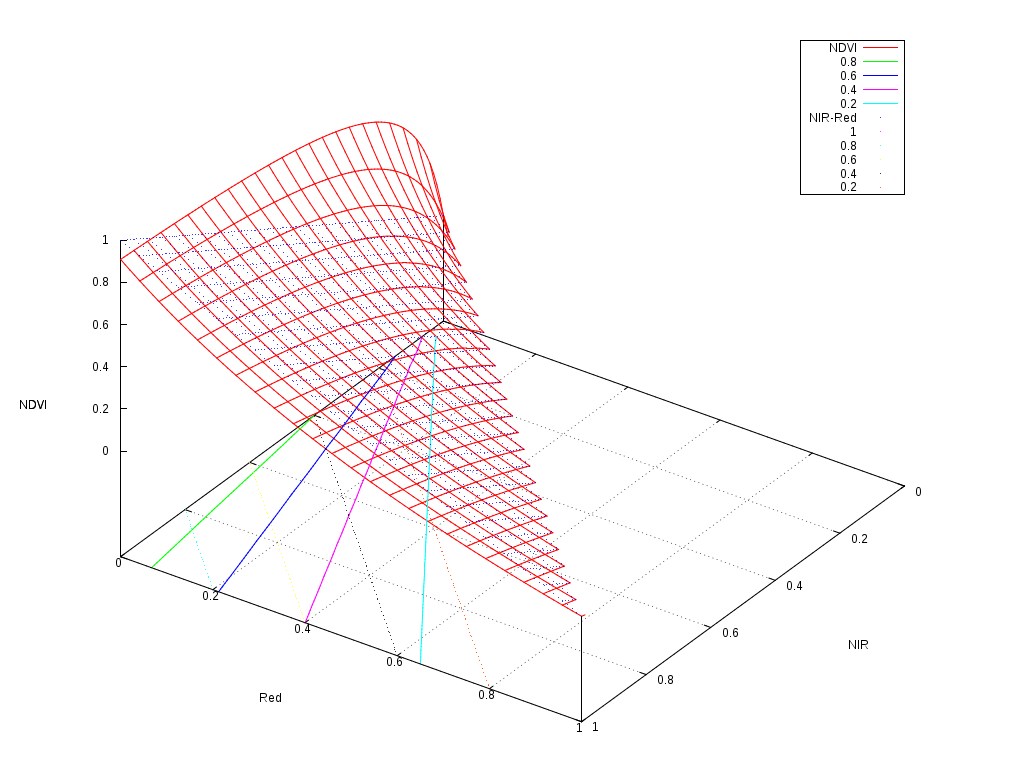
As one can see, it follows a plane with a slight non-linearity for the low reflectances. The contour plots are the solid colour lines, which are rather linear. So why we find that classifications often work better when we use this kind of indices?

The answer seems to reside in the distortion of the dynamics of the values.

If we have a look at the floor of the picture, we can imagine how a classifier would work.

The simplest classifier, that is a binary thresholding of the reflectances could only build a decision function following the black dotted grid, that is boundaries perpendicular to the axis. A decision tree, is just a set of thresholds on the features, and therefore, it could model a decision function which would be composed of a step functions on this plane, but always perpendicular and parallel to the axis.

On the other hand, a linear perceptron or a linear SVM, could build a decision function which would correspond to any straight line crossing this plane. An example of these lines would be the colour dotted lines representing the \(NIR-Red\) values. Any linear combination of the features would work like this.

It seems therefore, that a linear classifier could draw a boundary between a pair of solid colour lines, and therefore efficiently split the feature space as if the NDVI was available.

The interesting thing to note is that the NDVI contour plots are nearly straight lines, but they are not parallel. This introduces a kind of non-linear normalisation of the features which makes the job of the classifier easier.

And what about non-linear classifiers like multi-layer perceptrons or Gaussian SVM? Do they need these non-linear indices? The theoretical answer is “no, they don't”. But the pragmatic answer should be “please, be nice to your classifier”.

Most of the learning algorithms in the literature are based on the optimisation of cost functions. The easier the problem to solve, the higher the chances to get a robust classifier. In the case of SVM, this will result into a larger margin. In the case of Neural Networks, this will lead to a lesser chance of over-fitting.

Another thing to take into account is that cost functions in machine learning problems are based on distances, and most of the time the Euclidean distance is used. It is therefore useful to tune the features in order to give them the appropriate weight into this distance. In other words, if vegetation presence is something which conveys useful information for the classification, use the NDVI so that your classifier knows that¹.

Finally, non-linear classifiers are usually more computationally expensive than linear ones, both at the learning and at the inference step. Therefore, it is usually more effective to put the intelligence in the design of the features and use a simpler classifier than using raw features and a very sophisticated classifier.

Of course, all this advice is derived from a mix of the knowledge of the algorithms and the experience in using them for a particular kind of problem: remote sensing image supervised classification for land cover map production. For other applications in computer vision (like object recognition) or other completely unrelated fields, the advice might be different.

Is open and free global land cover mapping possible?

Short answer: yes.

Mid November took place in Toulouse "Le Capitole du libre", a conference on Free Software and Free Culture. The program this year was again full of interesting talks and workshops.

This year, I attended a workshop about contributing to Openstreetmap (OSM) using the JOSM software. The workshop was organised by Sébastien Dinot who is a massive contributor to OSM, and more importantly a very nice and passionate fellow.

I was very happy to learn to use JOSM and did 2 minor contributions right there.

During the workshop I learned that, over the past, OSM has been enriched using massive imports from open data sources, like for instance cadastral data bases from different countries or the Corine Land Cover data base. This has been possible thanks to the policies of many countries which have understood that the commons are important for the advancement of society. One example of this is the European INSPIRE initiative.

I was also interested to learn that what could be considered niche data, like agricultural land parcel data bases as for instance the French RPG have also been imported into OSM. Since I have been using the RPG at work for the last 4 years (see for example here or here), I was sympathetic with the difficulties of OSM contributors to efficiently exploit these data. I understood that the Corine Land Cover import was also difficult and the results were not fully satisfactory.

As a matter of fact, roads, buildings and other cartographic objects are easier to map than land cover, since they are discrete and sparse. They can be pointed, defined and characterised more easily than natural and semi-natural areas.

After that, I could not avoid making the link with what we do at work in terms of preparing the exploitation of upcoming satellite missions for automatic land cover map production.

One of our main interests is the use of Sentinel-2 images. It is the week end while I am writing this, so I will not use my free time to explain how land cover map production from multi-temporal satellite images work: I already did it in my day job.

What is therefore the link between what we do at work and OSM? The revolutionary thing from my point of view is the fact that Sentinel-2 data will be open and free, which means that the OSM project could use it to have a constantly up to date land cover layer.

Of course, Sentinel-2 data will come in huge volumes and a good amount of expertise will be needed to use them. However, several public agencies are paving the road in order to deliver data which is easy to use. For instance, the THEIA Land Data Centre will provide Sentinel-2 data which is ready to use for mapping. The data will be available with all the geometric and radiometric corrections of the best quality.

Actually, right now this is being done, for instance, for Landsat imagery. Of course, all these data is and will be available under open and free licences, which means that anyone can start right now learning how to use them.

However, going from images to land cover maps is not straightforward. Again, a good deal of expertise and efficient tools are needed in order to convert pixels into maps. This is what I have the chance to do at work: building tools to convert pixels into maps which are useful for real world applications.

Applying the same philosophy to tools as for data, the tools we produce are free and open. The core of all these tools is of course the Orfeo Toolbox, the Free Remote Sensing Image Processing Library from CNES. We have several times demonstrated that the tools are ready to efficiently exploit satellite imagery to produce maps. For instance, in this post here you even have the sequence of commands to generate land cover maps using satellite image time series.

This means that we have free data and free tools. Therefore, the complete pipeline is available for projects like OSM. OSM contributors could start right now getting familiar with these data and these tools.

Head over to CNES servers to get some Landsat data, install OTB, get familiar with the classification framework and see what could be done for OSM.

It is likely that some pieces may still be missing. For instance, the main approach for the map production is supervised classification. This means that we use machine learning algorithms to infer which land cover class is present at every given site using the images as input data. For these machine learning algorithms to work, we need training data, that is, we need to know before hand the correct land cover class in some places so the algorithm can be calibrated.

This training data is usually called ground truth and it is expensive and difficult to get. In a global mapping context, this can be a major drawback. However, there are interesting initiatives which could be leveraged to help here. For instance, Geo-Wiki comes to mind as a possible source of training data.

As always, talk is cheap, but it seems to me that exciting opportunities are available for open and free quality global mapping. This does not mean that the task is easy. It is not. There are many issues to be solved yet and some of them are at the research stage. But this should not stop motivated mappers and hackers to start learning to use the data and the tools.

Reproducible research

I have recently implemented the Spectral Rule Based Landsat TM image classifier described in ¹.

This paper proposes a set of radiometric combinations, thresholds and logic rules to distinguish more than 40 spectral categories on Landsat images. My implementation is available in the development version of the Orfeo Toolbox and should be included in the next release:

• Landsat Indices
• Landsat Classifier

One interesting aspect of the paper is that all the information needed for the implementation of the method is given: every single value for thresholds, indexes, etc. is written down in the paper. This was really useful for me, since I was able to code the whole system without getting stuck on unclear things or hidden parameters. This is so rarely found in image processing literature that I thought it was worth to post about it. But this is not all. Once my implementation was done, I was very happy to get some Landsat classifications, but I was not able to decide whether the results were correct or not. Since the author of the paper seemed to want his system to be used and gave all details for the implementation, I thought I would ask him for help for the validation. So I sent an e-mail to A. Baraldi (whom I had already met before) and asked for some validation data (input and output images generated by his own implementation). I got something better than only images. He was kind enough to send me the source code of the very same version of the software which was used for the paper – the system continues to be enhanced and the current version seems to be far better than the one published. So now I have all what is needed for reproducible research:

1. A clear description of the procedure with all the details needed for the implementation.
2. Data in order to run the experiments.
3. The source code so that errors can be found and corrected.

I want to publicly thank A. Baraldi for his kindness and I hope that this way of doing science will continue to grow. If you want to know more about reproducible research, check this site.

Change detection of soil states

As I mentioned in a previous post, last September I participated to the Recent Advances in Quantitative Remotes Sensing Symposium. I presented several posters there. One of them was about the work done by Benoît Beguet for his master thesis while he was at CESBIO earlier this year. The goal of the work was to assess the potential of high temporal and spatial resolution multispectral images for the monitoring of soil states related to agricultural practices. This is an interesting topic for several reasons, the main ones being:

1. a bare soil map at any given date is useful for erosion forecast and nitrate pollution estimations
2. the knowledge about the dates of different types of agricultural soil work can give clues about the type of crop which is going to be grown

The problem was difficult, since we used 8 m. resolution images (so no useful texture signature is present) and we only had 4 spectral bands (blue, green, red and near infrared). Without short-wave infra-red information, it is very difficult to infer something about the early and late phases.However, we obtained interesting results for some states and, most of all, for some transitions – changes – between states. You can have a look at the poster we presented at RAQRS here.

Geospatial analysis and Object-Based image analysis

I was searching in the web about the use of PostGIS data bases for object based image analysis (OBIA) and Google sent me to the OTB Wiki to a page that I wrote 6 months ago (first hit for "postgis object based image analysis").

It seems that this is a subject for which no much work is ongoing. Julien Michel will be presenting some results about how to put together OBIA and geospatial analysis (+ active learning and some other cool things) in a workshop in Paris next May.